Hurricane forecasting
In decades past, meteorologists had difficulty forecasting hurricanes. Occasionally, these massive supersystems would form, build and strengthen hundreds of miles offshore and then eventually strike coastal communities with startling violence. Given our lack of technology, the accuracy of identifying areas of landfall was far too imprecise, and thereby lessened the urgency of evacuation or preparedness directives. Over time, research and technology improved, giving us a better understanding of the forces behind these storms, and allowing us to better anticipate the timing and path of their arrival.
Significant progress was made with the development of early warning systems. These systems use sophisticated computer modeling to analyze vast amounts of data collected from radar and satellites. The goal of these efforts is to better forecast hurricanes by understanding the conditions conducive to their formation — relative humidity, gusting winds and elevated temperatures.
Aspiriant’s early warning system
Like the advances made by scientists in understanding natural disasters, professional investors have made significant strides in anticipating financial disasters. For example, we have developed a financial forecasting framework,1 which allows us to better assess and anticipate when the investment environment is likely attractive or challenging. More recently, we have improved the system,2 supplementing the forecasting analysis with ongoing monitoring systems.
Our framework has enabled us to develop a robust understanding of how economic and financial market cycles work. While many variables come into play, three factors tend to dictate the relative attractiveness of an investment environment: government (monetary and fiscal) stimulus, overconfidence and speculative investments.
Government stimulus
A government has an ability to affect the overall stimulus, either in financial liquidity or aggregate spending, across an economy. It can do so by changing its fiscal and/or monetary policies. If the combined policies are accommodative, the financial system is in a state of easing, with ample liquidity leading to faster economic growth. If the combined policies are restrictive, the financial system is in a state of tightening, with limited liquidity leading to slower economic growth.
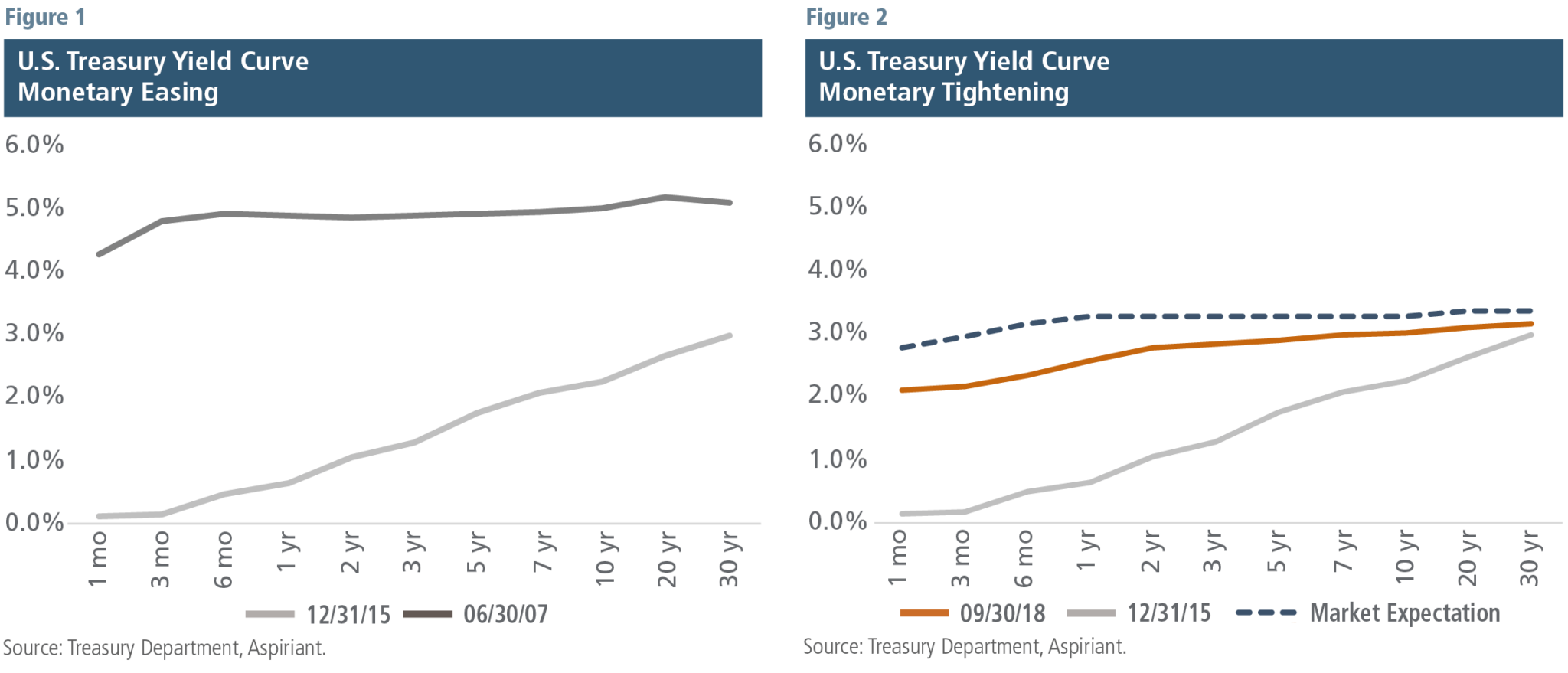
For example, from a monetary perspective, the U.S. Federal Reserve Board has the ability to influence liquidity in the financial system by decreasing or increasing interest rates. Figure 1 shows the dramatic steps taken by the Fed to pull the economy out of the Global Financial Crisis (GFC). The significant reduction in interest rates (through the reduction in the federal funds rate and quantitative easing) ultimately affected most other forms of borrowing, including mortgage rates, business loans, auto loans and credit cards. These actions injected massive amounts of liquidity into the financial markets, which led to credit creation, resulting in higher economic growth and inflated asset values. While the Fed’s policies did positively bend the economic growth curve, the most pronounced effects have been in the financial markets where asset prices have gone up by 300% cumulatively versus a gain of 20% in real gross domestic product.3
Once the economy was back on stable footing, the Fed shifted its policy stance by raising short-term rates beginning in December 2015 and trimming its holding of financial assets (U.S. Treasurys and mortgage-backed securities) in 2017. Figure 2 illustrates the unwinding of the stimulus, with both short-term and long-term rates drifting upward. Moreover, the market, taking direction from Federal Reserve Chairman Jerome Powell, expects additional monetary tightening over the next year.
Just as lower interest rates encourage spending and investments, higher interest rates discourage spending and investments. So, given the shift in the Fed’s policy, we expected higher interest rates to restrain economic growth. However, as monetary tightening was gaining momentum, Congress passed the Tax Cuts and Jobs Act at the end of 2017. This legislation dramatically reduced corporate tax rates and offered generous provisions to encourage investment and spending. By animating economic activity, fiscal policy changes temporarily served to offset and delay the effects of tighter monetary policy. But as the transient uplift in economic activity recedes over the next few quarters, we foresee a much more challenging environment, both in the real economy and in financial markets.
Interestingly, the parts of the economy more sensitive to interest rates have already started to bear the brunt of increasing financing costs. Over the past 12 months, home and auto purchases declined 1.5%4 and 4%5. Additionally, markets outside the U.S., without the ameliorating effects of fiscal stimulus, posted negative returns year-to-date as dollar funding costs (the world’s reserve currency) rose.
Overconfidence
So, changes in the level of government stimulus influence both the real economy as well as financial markets. However, the level of consumer and investor confidence exacerbates the impact. In general, increasing (decreasing) stimulus leads to more (less) confidence, which leads to more (less) risk-taking.
For example, when liquidity is plentiful, interest rates are low and consumer confidence is high, it typically leads to accelerated spending and strengthening economic conditions. However, contrary to common perceptions, buoyant consumer confidence doesn’t necessarily lead to attractive equity returns. In fact, our research6 has found that high levels of consumer confidence are typically followed by low levels of equity returns. Currently, consumer confidence7 is about as high as it was in September 1999. Over the following seven years through September 2006, the S&P 500 generated a modest annualized return of just 2.2%. Today, we forecast an annualized return of just 0.7% over the next seven years.
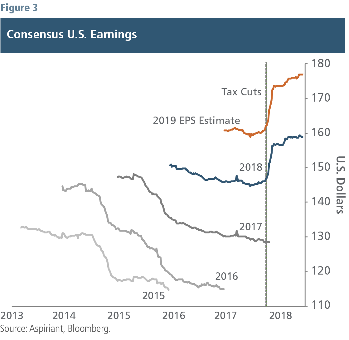
Like consumer confidence, high levels of investor confidence also tend to coincide with lower-than-expected future equity returns. Figure 3 presents the consensus earnings estimates across equity analysts for the S&P 500. For example, the light gray line tracks the changes in expected earnings starting in 2013 and continuing until the end of 2015, when actual 2015 earnings were reported by the 500 companies. A line that moves down indicates progressively lower earnings estimates. Conversely, a line that ends higher than its starting point suggests more optimism and confidence in corporate performance.
A key takeaway from the chart is that analyst expectations were consistently revised lower for forecasted earnings in 2015, 2016, 2017 and for much of 2018. Then, the Tax Cuts and Jobs Act was passed in December 2017. It seems quite logical that the impact should result in higher corporate earnings. However, what’s odd to us is that analysts appear to be extrapolating forward a continuing healthy (~10%) increase in future earnings, particularly in light of record profit margins. While above-trend revisions are understandable in the immediate aftermath of the passage of the legislation, we believe the longer-term projection is yet another sign of prevailing confidence and a dangerous extrapolation of short-term trends into the future.
Speculative investments
Overconfidence tends to lead to speculation, which can be extremely dangerous, especially in the late stages of a market cycle. For example, we have written extensively about the prevailing, and we believe unsustainably, high levels of equity valuations.8 However, many other examples of extreme risk-taking are evident in the financial system.
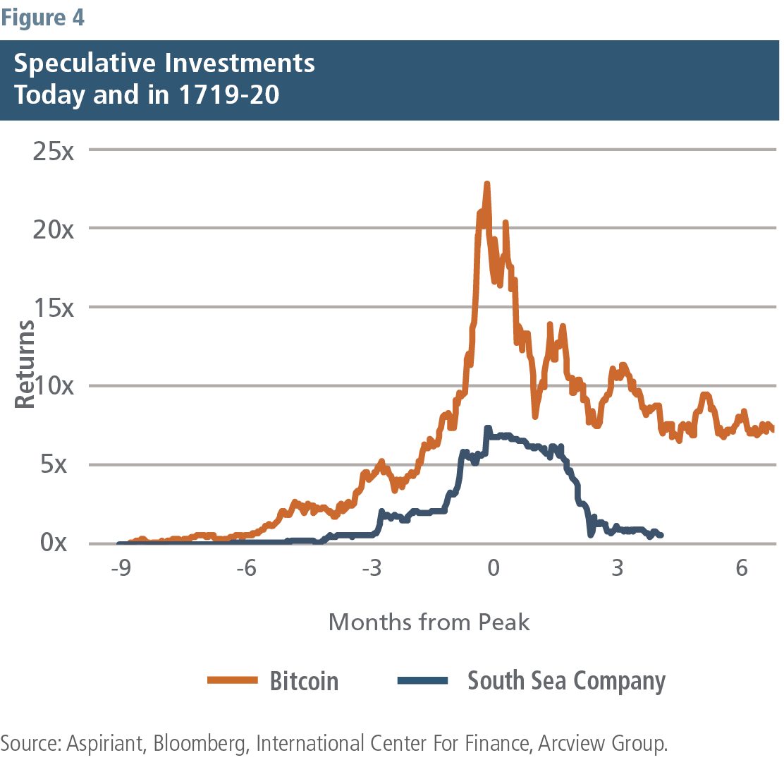
For example, Figure 4 compares the investment multiples of Bitcoin to the South Sea Company, which financially ruined Sir Isaac Newton.9 Although these bubbles occurred nearly 300 years apart, they have a few common features. First, they each show a clear building and bursting of a bubble. Second, they both have been characterized as speculative, with investors carelessly piling in without first evaluating the underlying risk and opportunity. Third, the building phase lasted about twice as long as the bursting phase.
Bubbles like bitcoin are emblematic of extreme risk-taking, especially during late-stage bull markets. To illustrate the point, according to Google Trends, the term “bitcoin” was the second most searched term in the global news category during 2017. By year-end, among the most frequent combined search terms were “buying bitcoin in my IRA” and “buying bitcoin with my credit card.” Moreover, nearly 75% of bitcoin holders could not identify a sound financial reason for investing in the cryptocurrency.10
Over the past several months, speculation seems to have given way to pragmatism as cryptocurrencies have lost nearly $600 billion in market capitalization.11 We suspect the losses will be felt by some retirees and consumers for quite some time to come.
Financial forecasting ≠ market timing
In late 2014, we wrote an Insight,12 entitled, “Preparing for Stormy Seas.” At that time, our analysis indicated that valuations of virtually all financial assets were above fair value, meaning expected returns would be lower going forward. In the letter, we argued that the tailwinds propelling the market upward would likely become headwinds. We concluded by advising investors to expect less return from their portfolios along with more volatility going forward. Given our outlook, we began positioning our portfolios toward a defensive posture. We reduced global equities, tilting our portfolios toward defensive equities, defensive strategies and fixed income.
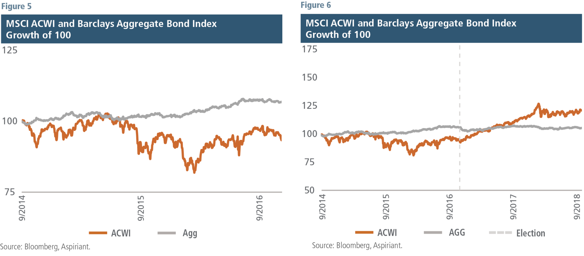
So, how did our advice playout? For simplification, Figure 5 compares global equities and fixed income between September 2014 and September 2016. During that time, global equities were indeed volatile, losing 6.7%, whereas fixed income was stable, gaining 6.9%. As a result, an underweight to global equities was a wise decision.
However, as shown in Figure 6, the relationships reversed between September 2016 and September 2018. Anticipation of fiscal policy changes following the U.S. presidential election, combined with higher (albeit modest) global economic growth, buoyed all risk assets in 2017. While the fiscal policy changes prolonged the bull market by another two years, we expect the impact to fade in the coming quarters. In fact, our forecasted return for global equities and fixed income are approximately the same at 2.2% annualized over the next seven years. However, we expect global equities to have approximately 3.5x the amount of risk. So, it’s certainly plausible that equities could well underperform fixed income, especially since they tend to be extremely sensitive to changes in interest rates (discount rates) and reversals in economic conditions. Accordingly, a world with resetting (higher) interest rates and slowing growth is not well positioned for strong equity market performance.
Dialing in economic and market currents
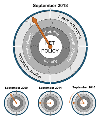
Understanding the impact of government stimulus on economic growth as well as asset valuations is critical to understanding what’s more likely or less likely to occur in the future. Government stimulus has a direct relationship with economic growth and an indirect relationship with asset valuations. The diagram below illustrates the connections.
September 2018
Starting with the dark gray circle, a government uses monetary policy to either promote or dampen economic growth. For instance, the Fed can either increase or decrease short-term interest rates by changing the federal funds rate. It can also increase or decrease long-term rates through asset purchases and sales. The impact of these monetary decisions will change both the height and slope of the yield curve, which ultimately determines virtually all other borrowing rates for consumers and businesses.
Therefore, monetary policies encourage or discourage credit creation, which impacts economic growth. As illustrated by the medium gray circle, monetary policy usually has a lagged effect on the economy, especially for unconventional policies like quantitative easing. In general, the Fed starts to tighten while growth is rising and continues doing so even after growth has begun to slow. Similarly, the Fed tends to “overshoot” during periods of easing as well, pursuing stimulative actions even after growth starts rising.
In changing its policy decisions, the Fed monitors a variety of economic variables, perhaps the two most important of which are unemployment and inflation. But, while it has no stated objective of influencing asset prices, its decisions most certainly have a flow-through effect on financial asset valuations. Valuations, specifically the growth rate of real (inflation-adjusted) cash flows and the discount rate to compute the present value of those cash flows, are inseparably shaped by Fed policies. As illustrated by the light gray circle, as tightening begins, economic growth is often still rising, but asset valuations begin to fall. That’s because investors begin to anticipate the slowing economy and the change in the present value of the cash flows ascribed to various securities, even before they occur.
Other periods
By our estimates, the overall macroeconomic environment today is quite similar to September 2000, a period in which tightening had begun, growth was plateauing, and asset prices began to fall. We have also illustrated where we were in September 2014, which is why we began to move toward a more defensive positioning. But then, in September 2016, as we approached the end of the current market cycle, corporate cash repatriation and tax cuts effectively served to “rewind the clock” to September 2014’s positioning, extending the bull market a couple more years.
As we mentioned, we expect those impacts to be transitory in nature and believe they have already begun to dissipate. While public policy can delay the inevitable, it cannot serve to avoid it. The forces driving economic and market currents are simply too strong to subdue.
What keeps us up at night?
Since our portfolios are defensively positioned, we expect to outperform in the event of a market downturn. So, what “keeps us up at night” is a scenario in which the market continues to march irrationally higher, causing our portfolios to underperform their passive benchmarks. While a valid concern, we have identified just three catalysts that could lead to that outcome (ranked from highest efficacy to lowest):
1. The Fed changes course on its path to policy normalization and instead reduces (or to a lesser degree maintains) current interest rates
2. The passing of a large-scale fiscal spending plan, potentially to improve the country’s infrastructure
3. Quickly and favorably resolving global trade disputes, especially with China
While any of these circumstances could occur, we believe the probability is remote. Moreover, any of them would likely only stave off a market pullback for another year or two, at which point a downturn would likely be ever more severe.
In fact, as we were going to press with this Insight, global equities sold off sharply, declining 8% over the first several trading days in October. Adding that data onto Figure 6 strengthens the case for the stable, predictable performance of fixed income. Moreover, we believe the forces leading to the selloff in equities will persist and grow in coming months, indicative of late-stage dynamics across financial markets.
No portfolio would be impervious to a widespread financial retreat. However, we expect globally diversified, defensively positioned portfolios to compare favorably. Therefore, we feel well-positioned for such an environment and look forward to the opportunity to redeploy our defensive assets into riskier assets as they become attractively priced.
Footnotes:
1We refer to our forecasting outputs as Capital Market Expectations (CMEs) and monitoring tools as financial EKGs.
2For a broader discussion, see our Insight, Capital Market Expectations, March 2016
3From 12/31/2008 to 9/30/2018.
4Source: National Association of Realtors.
5Source: Bureau of Economic Analysis.
6See our Q3 2017 Insight.
7Source: Michigan Consumer Confidence Index.
8For a broader discussion, please see our Insights published in Q4 2017, Q1 2018 and Q2 2018.
9For a broader discussion, please see our Foundational Elements: Speculator or Investor?
10Source: MarketWatch.
11Source: Cryptocurrency News. After peaking at a market capitalization of $850 billion in December 2017, cryptocurrencies are collectively worth approximately $250 billion today.
12See Preparing for Stormy Seas, December 2014.
Illustration by Ken Cummings
Important disclosures
Past performance is no guarantee of future performance. All investments can lose value. Indices are unmanaged and you cannot invest directly in an index. The volatility of any index may be materially different than that of a model. The charts and illustrations shown are for information purposes only.
Equities. The S&P 500 is a market-capitalization weighted index that includes the 500 most widely held companies chosen with respect to market size, liquidity and industry. The Dow Jones Internet Commerce Index (eCommerce) is designed to measure the 15 largest and most actively traded internet commerce stocks. The MSCI ACWI Index is a free float-adjusted market capitalization weighted index that is designed to measure the equity market performance of developed and emerging markets.
Fixed Income. The Barclays U.S. Aggregate Index represents securities that are SEC-registered, taxable and dollar denominated. The index covers the U.S. investment grade fixed rate bond market, with index components for government and corporate securities, mortgage pass-through securities and asset-backed securities. These major sectors are subdivided into more specific indices that are calculated and reported on a regular basis.

 Talk to us

